Session 1.3

Immortal time bias

Louisa Smith

Recap

Not everyone will ultimately be at risk for many outcomes of interest due to competing events
- If we have information on them, there are still causal estimands of interest
Not everyone will be identified/enroll in a study because they have a competing event before that point, in which case we don’t have information on them (left truncation)
- When this is random with respect to the exposure and outcome, we can correct for it
- When it is differential with respect to the exposure, we need to think more carefully…

Now let’s think about an exposure that doesn’t occur at the same time for everyone

e.g., vaccination during pregnancy

It’s still a one-time treatment (let’s assume for simplicity!)
But it can happen at different times during pregnancy for different people

Again we will generate it under the sharp null hypothesis

dat <- dat |> 
  mutate(
    time_potentially_exposed = runif(n(), 0, 45),
    time_potentially_exposed = to_weeks_days(time_potentially_exposed),
    time_exposed = ifelse(
      time_potentially_exposed < gest_week,
      time_potentially_exposed,
      NA
    ),
    week_exposed = floor(time_exposed),
    ever_exposed = ifelse(!is.na(time_exposed), 1, 0),
    # Set time_exposed to arbitrarily high value if never exposed
    # to not have to deal with NAs in later analyses
    time_exposed = ifelse(is.na(time_exposed), 1000, time_exposed),
    week_exposed = ifelse(is.na(week_exposed), 1000, week_exposed)
  )

Randomly assigned exposure time

The code is explained more in the exercises, but basically:

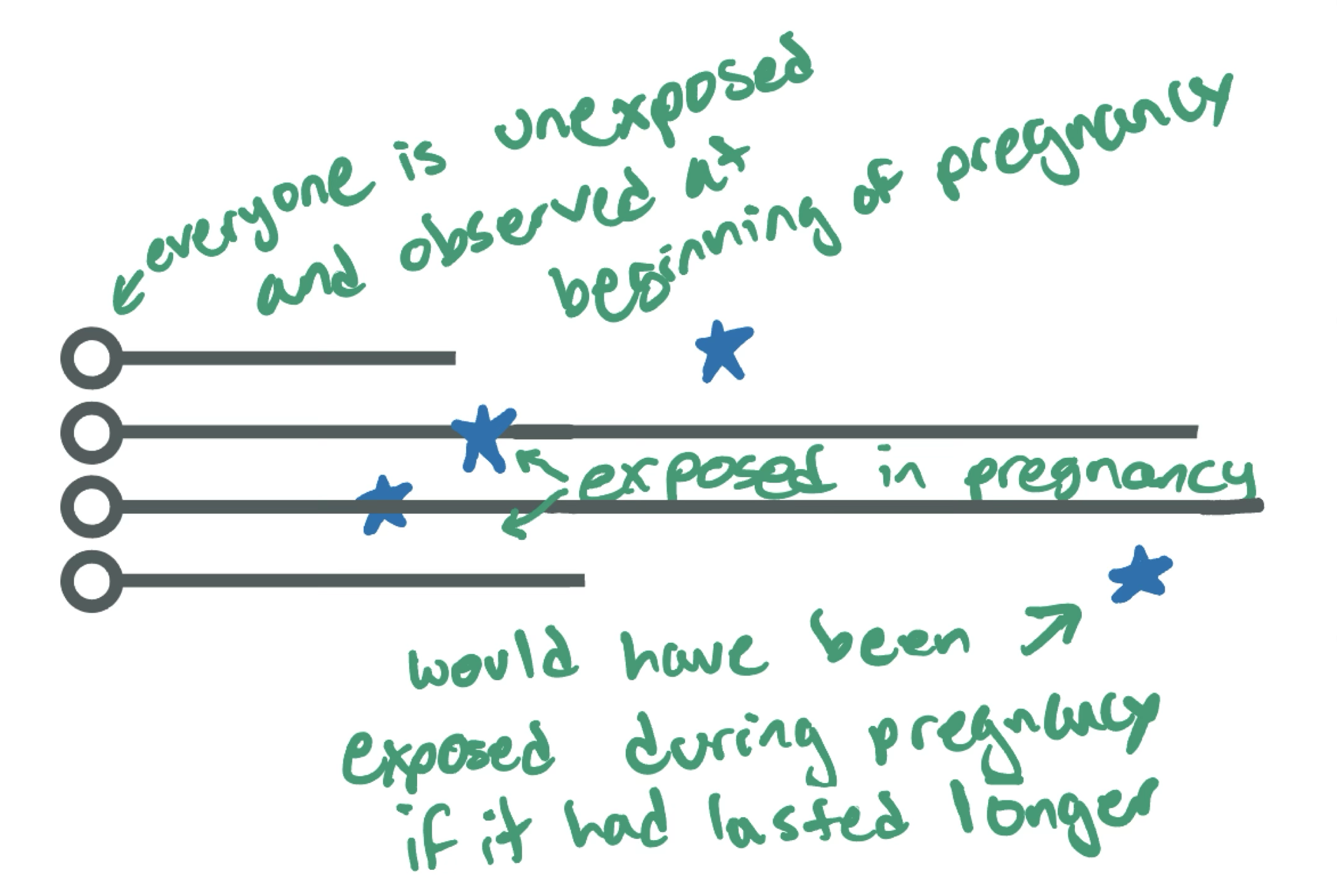
Everyone has a random time when they could be exposed (uniformly distributed between 0 and 45 weeks)
If that time is before the pregnancy ends, they are considered exposed at that time
If that time is after the pregnancy ends, they are considered never exposed

We are still generating data under the null hypothesis (no effect of exposure on outcome for any individual)

Let’s look at some summary statistics

Variable	Unexposed N = 3,048¹	Exposed N = 6,952¹	Total N = 10,000¹
Spontaneous abortion (<20 weeks gestation)
0	1,039 (34%)	6,365 (92%)	7,404 (74%)
1	2,009 (66%)	587 (8.4%)	2,596 (26%)
Child born preterm or less than 37 weeks as yes and no
0	783 (75%)	5,718 (90%)	6,501 (88%)
1	256 (25%)	647 (10%)	903 (12%)
Unknown	2,009	587	2,596
¹ n (%)

Wait…

I said exposure could happen throughout pregnancy, but spontaneous abortion (SAB) can only happen before 20 weeks

Restricting to a relevant exposure window doesn’t solve the problem

Variable	Unexposed N = 3,048¹	Exposed before 20 weeks N = 3,827¹	Total N = 6,875¹
Spontaneous abortion (<20 weeks gestation)
0	1,039 (34%)	3,240 (85%)	4,279 (62%)
1	2,009 (66%)	587 (15%)	2,596 (38%)
Child born preterm or less than 37 weeks as yes and no
0	783 (75%)	2,847 (88%)	3,630 (85%)
1	256 (25%)	393 (12%)	649 (15%)
Unknown	2,009	587	2,596
¹ n (%)

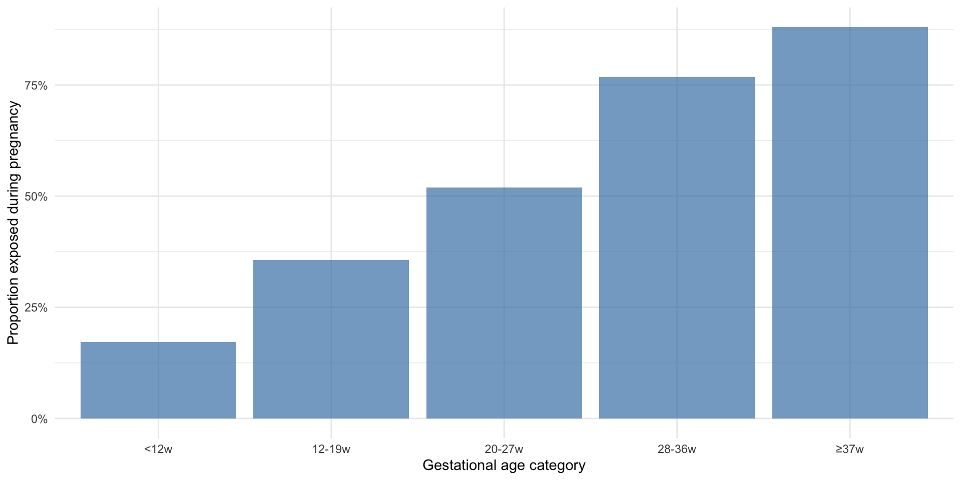
Shorter pregnancies are less likely to be exposed

The bias

People who are exposed have by definition a pregnancy that lasted long enough to be exposed (whenever that is)
So exposed group is more likely to be “immortal” (cannot have the outcome) during the time before exposure
- Simpler examples of immortal time bias might compare, e.g., no treatment vs. two years of treatment (must survive that long)

Immortal time bias

Suissa (2008) is probably the most commonly cited description

Several recent papers attempting to describe it structurally, including Mansournia, Nazemipour, and Etminan (2021); Yang, Burgess, and Schooling (2025); Hernán et al. (2025)

Immortal time bias

The term “immortal time bias” suggests that the source of the bias is the immortal time, but it is selection or misclassification that generates the immortal time, leading to bias.

The difference is whether observations not surviving the “immortal time” are preferentially excluded (selection), or just classified as unexposed (misclassification)

Immortal time biases in pregnancy

Selection (“post-assignment eligibility”)
- e.g., restricting to people with pregnancies lasting at least 20 weeks, when exposure can happen earlier (i.e., had a competing event before joining the study – left truncation)
  - this is a problem whether you start follow-up at 20 weeks or look back and start it earlier
  - (this is not a problem if your exposure happens after 20 weeks)
Misclassification (“post-eligibility assignment”)
- e.g., classifying pregnancies as exposed after surviving to exposure, even though exposure didn’t occur at baseline

‎

“assignment” here refers to treatment assignment, or exposure timing

Immortal time due to selection

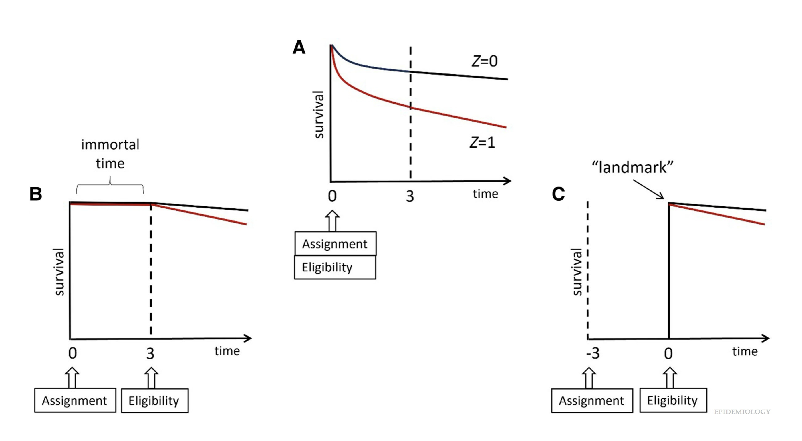
Survival curves from a follow-up study based on all data (A), on data restricted to those who survive at least 3 months with follow-up starting at assignment (B), and on data restricted to those who survive at least 3 months with follow-up starting at 3 months (C). (Hernán et al. 2025)

Immortal time due to misclassification

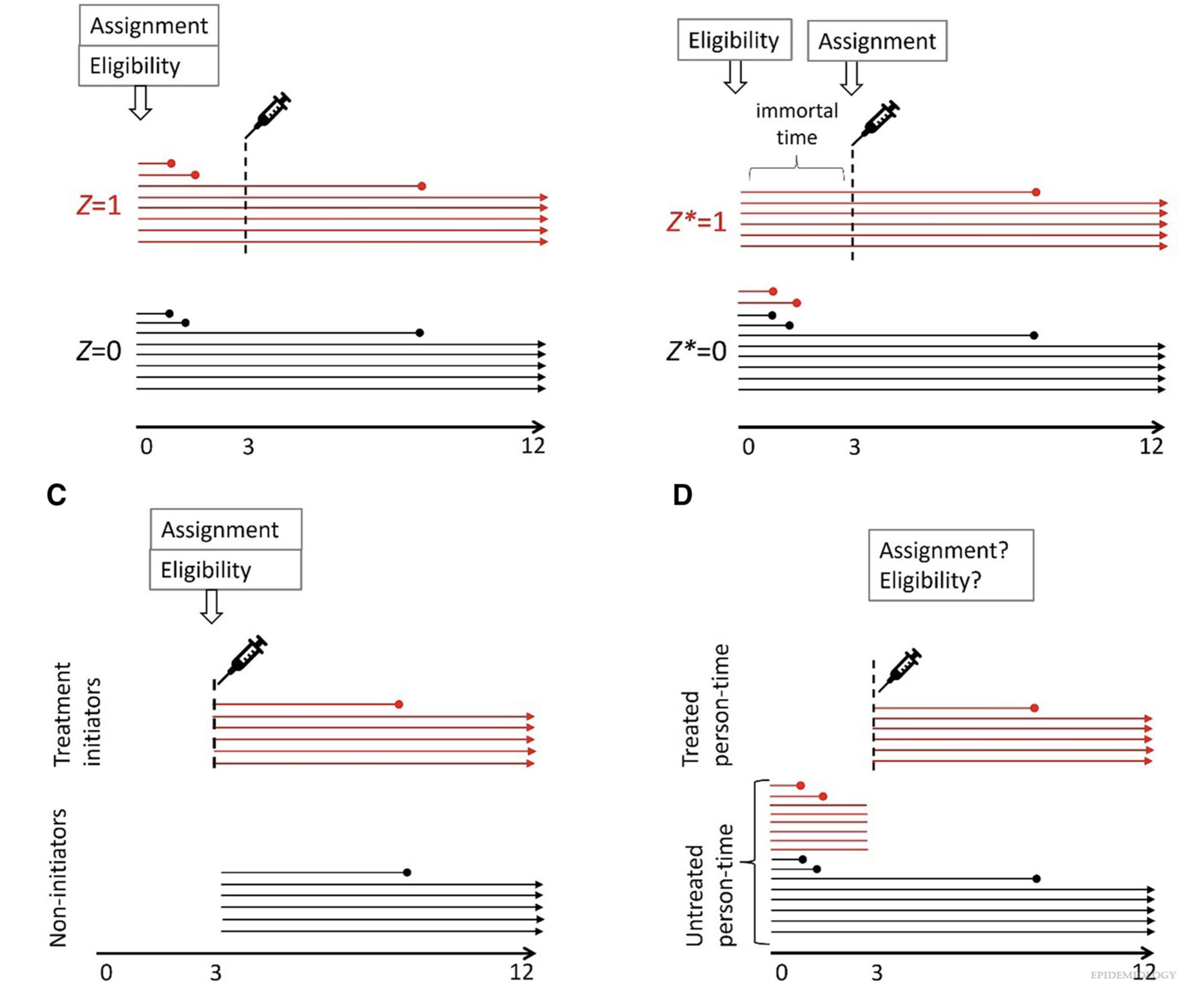
Schematic representation of a study with 16 individuals (horizontal lines) assigned to one of two strategies indistinguishable at time zero: (A) original assignment Z, (B) reconstructed assignment Z* with immortal time, (C) reconfiguration of the data to emulate a study in which individuals are assigned to strategies that are distinguishable at time zero (no immortal time), and (D) reconfiguration of the data to allocate person-time to “exposed” and “unexposed” categories (no immortal time). (Hernán et al. 2025)

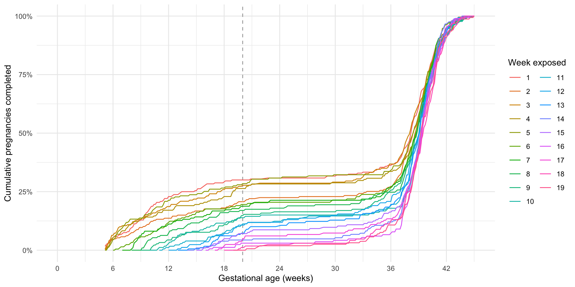
What if we are only interested in exposed pregnancies and we have everyone’s data?

We saw that left truncation was a problem when pregnancies had already ended before enrolling or being identified in a study

The same thing happens even if everyone is enrolled at the start of pregnancy, but we are comparing exposed pregnancies to each other based on timing of exposure

This means that we can’t even tell whether there is an effect of timing of exposure

Let’s look at what the risk of SAB is by week of exposure

exposure_timing_risk <- dat |>
  # only include those exposed before SAB cutoff
  filter(week_exposed < 20) |> 
  # calculate risk of SAB separately for each week of exposure
  group_by(week_exposed) |>
  summarise(pr_sab = mean(sab))

The risks are variable, but as expected, they decrease with gestational age

Remember that we generated data under the null hypothesis (no effect of exposure on outcome for any individual)

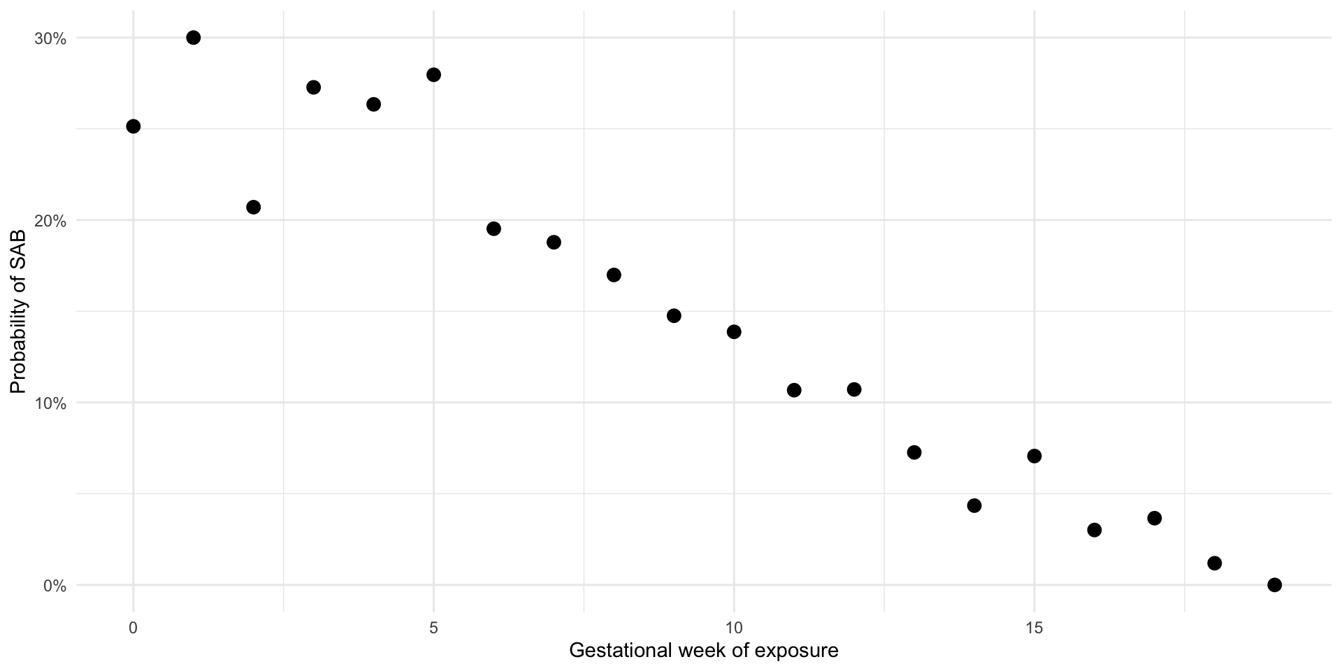
Cumulative incidence of SAB by week of exposure

What if we compare exposed to unexposed but still pregnant?

We can compare pregnancies exposed in week 6 to those still pregnant but unexposed in week 6
We can compare pregnancies exposed in week 7 to those still pregnant but unexposed in week 7
- This will include most of the previous comparison group
And so on…

Let’s think about what this looks like

Who will be in each group for a comparison at week 6? Who will be in each group for a comparison at week 7?

ID	week_exposed	gest_week
1	6	34
2	7	18
3	32	40
4	1000	6.5
5	1000	36

‎

Recall that we have set week_exposed to 1000 for unexposed pregnancies

Comparisons

ID	week_exposed	gest_week
1	6	34
2	7	18
3	32	40
4	1000	6.5
5	1000	36

At week 6:
- Exposed: ID 1
- Unexposed but still pregnant: ID 2, 3, 4, 5
At week 7:
- Exposed: ID 2
- Unexposed but still pregnant: ID 3, 5

How do we implement this in code?

Create a dataset for each week of pregnancy
In each dataset, classify people as exposed if they were exposed that week, unexposed if they are still pregnant but unexposed that week, and exclude if they already had the outcome or the pregnancy ended

Let’s do this for all weeks

We’ll use the crossing() function to create a dataset for each week of pregnancy (all concatenated together)

sab_weekly <- dat |>
  crossing(week_comparison = 6:19)
sab_weekly |> 
  select(ID, week_exposed, gest_week, week_comparison)

# A tibble: 140,000 × 4
      ID week_exposed gest_week week_comparison
   <int>        <dbl>     <dbl>           <int>
 1     1            7      40.6               6
 2     1            7      40.6               7
 3     1            7      40.6               8
 4     1            7      40.6               9
 5     1            7      40.6              10
 6     1            7      40.6              11
 7     1            7      40.6              12
 8     1            7      40.6              13
 9     1            7      40.6              14
10     1            7      40.6              15
# ℹ 139,990 more rows

Let’s do this for all weeks

Now we can remove 1) those who already had an event, and 2) those who already had an exposure (so they are either exposed that week, or still unexposed)

sab_weekly <- sab_weekly |>
    # still pregnant at trial time
  filter(gest_week >= week_comparison) |> 
  filter(
    # eligible at trial time (removing anyone exposed before the trial)
    week_exposed > week_comparison | # exposed never or later
    week_exposed == week_comparison  # exposed now
  ) |>
  mutate(
    # indicate whether exposed this week
    exposed_now = ifelse(week_exposed == week_comparison, 1, 0)
  )

Example individual

ID	week_exposed	gest_week	week_comparison	exposed_now
10281	7	38	6	0
10281	7	38	7	1

Example individual

ID	week_exposed	gest_week	week_comparison
26859	1000	8	6
26859	1000	8	7
26859	1000	8	8

Example individual

ID	week_exposed	gest_week	week_comparison
2589	1000	38	6
2589	1000	38	7
2589	1000	38	8
2589	1000	38	9
2589	1000	38	10
2589	1000	38	11
2589	1000	38	12
2589	1000	38	13
2589	1000	38	14
2589	1000	38	15
2589	1000	38	16
2589	1000	38	17
2589	1000	38	18
2589	1000	38	19

We can see the expected patterns in sample size across comparisons

week_comparison	n_0	n_1
6	8169	210
7	7689	197
8	7247	206
9	6871	183
10	6514	173
11	6182	178
12	5895	168
13	5617	179
14	5342	207
15	5082	184
16	4862	166
17	4636	164
18	4411	168
19	4209	158

Now we can compare

# Calculate risks by week
sab_risks_weekly <- sab_weekly |>
  group_by(week_comparison, exposed_now) |>
  summarise(pr_sab = mean(sab))

sab_risks_weekly

# A tibble: 28 × 3
# Groups:   week_comparison [14]
   week_comparison exposed_now pr_sab
             <int>       <dbl>  <dbl>
 1               6           0  0.230
 2               6           1  0.195
 3               7           0  0.203
 4               7           1  0.188
 5               8           0  0.178
 6               8           1  0.170
 7               9           0  0.156
 8               9           1  0.148
 9              10           0  0.132
10              10           1  0.139
# ℹ 18 more rows

All comparisons

Believe it or not this is still not an entirely fair comparison!

This will motivate target trial emulation and the clone-censor-weighting approach in the next sessions

Hernán, Miguel A., Jonathan A. C. Sterne, Julian P. T. Higgins, Ian Shrier, and Sonia Hernández-Díaz. 2025. “A Structural Description of Biases That Generate Immortal Time.” Epidemiology 36 (1): 107. https://doi.org/10.1097/EDE.0000000000001808.

Mansournia, Mohammad Ali, Maryam Nazemipour, and Mahyar Etminan. 2021. “Causal Diagrams for Immortal Time Bias.” International Journal of Epidemiology 50 (5): 1405–9. https://doi.org/10.1093/ije/dyab157.

Suissa, Samy. 2008. “Immortal Time Bias in Pharmacoepidemiology.” American Journal of Epidemiology 167 (4): 492–99. https://doi.org/10.1093/aje/kwm324.

Yang, Guoyi, Stephen Burgess, and Catherine Mary Schooling. 2025. “Illustrating the Structures of Bias from Immortal Time Using Directed Acyclic Graphs.” International Journal of Epidemiology 54 (1): dyae176. https://doi.org/10.1093/ije/dyae176.