Session 1.2

Biases in pregnancy research

Louisa Smith

We need an exposure

• In the previous section, we looked at a simulated dataset with pregnancy outcomes
• Now we need to simulate an exposure
• We are going to randomly assign exposures to ensure that we’re operating under the sharp null hypothesis (no effect of exposure on outcome for any individual)

Null hypothesis

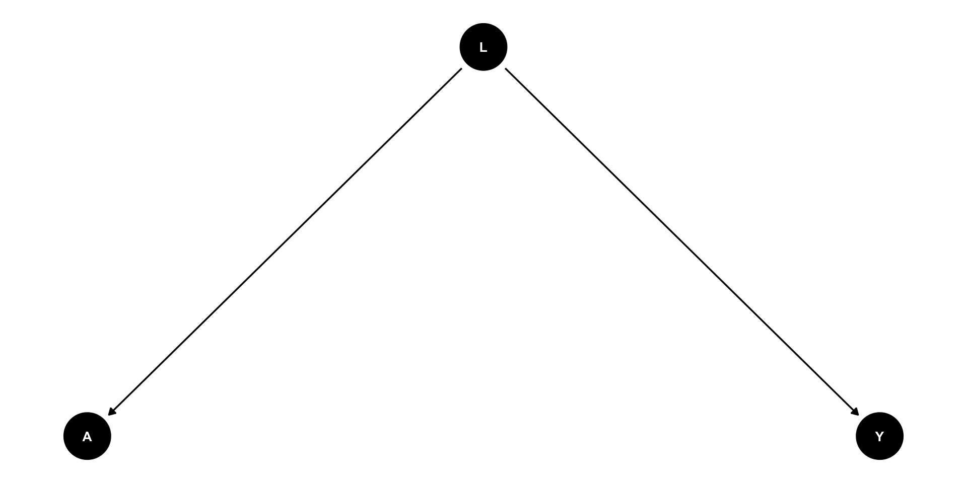
You’ll often see DAGs drawn under the null hypothesis (no arrow from exposure to outcome)

• This helps us see certain biases
• We can see conditions in which exposure and outcome are going to be associated even if there is no causal effect

Null hypothesis

When developing code, it can be helpful to simulate data under the null hypothesis (even if you have the real data!)

• I often write code that is wrong (like everyone, I think!) and only realize it when I see an effect where there shouldn’t be one

Let’s simulate a very simple exposure

• Assume it happens once during pregnancy (and only during pregnancy)
• At the same time for everyone (let’s say at 6 weeks, since our data start there)
• Everyone either has it or not
• We have data on everyone starting at the time of exposure

‎

This is basically a best-case scenario in pregnancy research!

Let’s simulate an exposure

dat <- dat |>
  mutate(
    treat = sample(c(0, 1), n(), replace = TRUE, prob = c(0.5, 0.5))
  )

count(dat, treat, stillbirth)

# A tibble: 6 × 3
  treat stillbirth     n
  <dbl>      <dbl> <int>
1     0          0  3635
2     0          1    73
3     0         NA  1334
4     1          0  3619
5     1          1    77
6     1         NA  1262

Two R functions we’ll use a lot

• mutate(data, new_var = f(var1, var2), ...): create or transform variables
• count(data, var1, var2, ...): count occurrences of combinations of variables

As we saw in the first set of exercises, we are using the pipe operator (|>) to pass a dataset to a function

• (We could also have said dat |> count(treat, stillbirth))

Problems with even a simple exposure

What if we are interested in an outcome that occurs later in pregnancy, but which cannot occur if the pregnancy ends early?

• Stillbirth is one such outcome – it is only defined for pregnancies that did not end in spontaneous or induced abortion

Similarly, what if we are interested in a pre-pregnancy exposure but not everyone becomes pregnant?

Conditioning on achieving pregnancy

• Many studies consider pre-pregnancy treatments or exposures
• The outcomes of interest often only occur in pregnant people
• Intuitively: treatment may affect conception, so when we are comparing outcomes in treated vs. untreated pregnant people, we are comparing different groups even if the treatment was randomized

Example: Fertility treatments and neonatal complications

• Treatments may affect both live birth probability AND neonatal outcomes
  • If treatment increases failure to conceieve and/or pregnancy loss, fewer complications observed
  • Not because treatment prevents complications, but prevents births

‎

Need to be clear about the estimand we’re targeting

Chiu et al. (2020)

Let’s distinguish a few types of events

• Loss to follow-up: the outcome of interest can occur but is not observed
  • Chose to stop participating
  • Moved away/can’t be contacted
  • Changed insurance/health systems
• Competing event: prevents the outcome of interest from occurring at all
  • Failure to conceive
  • Pregnancy loss
  • Death

‎

Sometimes “semi-competing” risks are distinguished (when only one event prevents the other, but not vice versa), as are “truncating” events, which prevent a total effect from being defined for a given outcome

Some estimands in the presence of competing event (\(D\))

Total effect: Effect of treatment on outcome, ignoring competing event

• Pregnancies/attempted pregnancies not ending in live birth are included in the denominator (but not the numerator)
• \(\Pr(Y^{a=1} = 1)\) vs. \(\Pr(Y^{a=0} = 1)\)

Some estimands in the presence of competing event (\(D\))

Composite effect: Effect of treatment on outcome OR competing event

• The outcome is defined to include any of failure to conceive, pregnancy loss, or complications of interest
• Pregnancies/attempted pregnancies not ending in live birth are included in both the numerator and denominator
• \(\Pr(Y^{a=1} \text{ or } D^{a=1} = 1)\) vs. \(\Pr(Y^{a=0} \text{ or } D^{a=0} = 1)\)

Some estimands in the presence of competing event (\(D\))

Controlled direct effect: Effect of treatment on outcome if competing event were eliminated

• Pregnancies/attempted pregnancies not ending in live birth are not included at all
• (This is probably what is most often done, whether purposeful or not)
• \(\Pr(Y^{a=1, d=0} = 1)\) vs. \(\Pr(Y^{a=0, d=0} = 1)\)

Pros and cons in interpretation

• Total effect: Makes sense if we care about the overall risk of the outcome in some population
  • For example, if preparing resources to deal with birth complications in a hospital, we care about the risk in the whole population of people who might become pregnant
• Composite effect: Makes sense if we care about the overall risk of any bad outcome, and the competing event is on the “same scale” as the outcome
  • It’s hard (and very subjective) to combine such outcomes (e.g., failure to conceive vs. birth complications that sill results in a live birth; failure to conceive vs. infant death)
• Controlled direct effect: Makes sense if we care about the etiology of the outcome, or if we want to understand the effect of treatment in a hypothetical world where the competing event does not occur
  • Perhaps we can imagine a future where that is possible

Pros and cons in interpretation

For an outcome like birthweight, these are truncating events

• The total effect and composite effects are not defined (what is the birthweight of a pregnancy that ends in miscarriage?)
• They worked for binary outcomes because we could combine their definitions with a binary competing event

Identifiability

Both total and composite effects are identifiable in randomized controlled trials (under standard assumptions)

• \(\Pr(Y^{a=1})\) vs. \(\Pr(Y^{a=0})\) (total effect)
• \(\Pr(Y^{a=1} \text{ or } D^{a=1})\) vs. \(\Pr(Y^{a=0} \text{ or } D^{a=0})\) (composite effect)

Controlled direct effects, however, are an intervention on both treatment and the competing event, which would require randomization of failure to conceive/pregnancy loss

• \(\Pr(Y^{a=1, d=0})\) vs. \(\Pr(Y^{a=0, d=0})\) (controlled direct effect)

Obviously we can’t randomize pregnancy loss

• Any analysis involving a competing event needs to think carefully about what estimand is of interest
• If it’s the controlled direct effect, confounding of the competing event-outcome relationship must be addressed
  • And the interpretation must be specific to the hypothetical world where the competing event does not occur

Other competing events estimands

• Separable effects: If the treatment can be decomposed into two components, one affecting the outcome and one affecting the competing event, we can consider effects of each component (Stensrud et al. 2020)
• Principal stratum effects: Effect of treatment on outcome in the subgroup who would not experience the competing event regardless of treatment (survivor average causal effects) (Rubin 2000)
• Stochastic direct effects: Effect of treatment on outcome if we could shift the distribution of the competing event (Gupta et al. 2024)

What about other competing risks analyses?

Subdistribution function, cause-specific hazards, etc.

Young et al. (2020) explains what statistical estimands correspond to causal estimands

Regression in R

We’ll use regression to estimate (a version of) each of the three estimands in the exercises

• Not worrying about identifiability (code includes a variety of covariates for adjustment, but not the focus of the exercise)
• The goal is to get comfortable with the syntax in R because we’ll be using regression for other analyses

Regression in R

# Linear regression
lm_model <- glm(
  birthweight ~ treat + maternal_age + BMI_b4preg,
  family = gaussian,
  data = dat
)

# Logistic regression 
logit_model <- glm(
  preterm ~ treat + maternal_age + BMI_b4preg,
  family = binomial,
  data = dat
)

We will see similar syntax (on the right-hand side) for survival analysis (e.g., Kaplan-Meier, Cox regression)

Regression in R

We can use the gtsummary package to make nice tables of results

tbl_regression(logit_model, exponentiate = TRUE)

Characteristic	OR	95% CI	p-value
treat	0.98	0.85, 1.12	0.7
Maternal age at the begining of pregnancy	1.00	0.99, 1.01	>0.9
Pre-pregnancy BMI	1.01	1.00, 1.02	0.2
Abbreviations: CI = Confidence Interval, OR = Odds Ratio

Creating and looking at new variables

dat <- dat |>
  mutate(
    # combining outcomes for composite effect
    sab_still = ifelse(sab == 1 | stillbirth == 1, 1, 0),
    # reclassifying NA as 0 for total effect
    still_total = ifelse(is.na(stillbirth) | stillbirth == 0, 0, 1)
  )

count(dat, sab, stillbirth, sab_still, still_total)

# A tibble: 3 × 5
    sab stillbirth sab_still still_total     n
  <dbl>      <dbl>     <dbl>       <dbl> <int>
1     0          0         0           0  7254
2     0          1         1           1   150
3     1         NA         1           0  2596

Exercises part 1

What if we don’t have data on the people who had the competing event?

We always have to worry about the fact that exposure may have affected who’s in the study (because they can’t have experienced a competing event to enroll or be identified in the data)

• This may be less of a problem in database studies where you can identify all pregnancies
  • But of course can’t generally identify all attempted pregnancies to study pre-pregnancy exposures
  • Many pregnancies are unplanned, so people don’t even know themselves if they were part of that population

Left truncation

• When there are some observations we only observe starting some time after baseline, we have left truncation
• In pregnancy research, this is often because we only observe people starting at pregnancy detection (e.g., first prenatal visit, first ultrasound)
• People find out they’re pregnant at different gestational ages

Let’s compare risks of spontaneous abortion assuming different patterns of enrollment

We have data on everyone starting at 6 weeks

dat_6wk <- dat |> filter(gest_week >= 6)

We have data on everyone starting at 12 weeks

dat_12wk <- dat |> filter(gest_week >= 12)

We can calculate the proportion of SAB in each dataset

summarise(dat_6wk, risk = mean(sab))
summarise(dat_12wk, risk = mean(sab))

Another helpful R function

• summarise() (or summarize()): create whatever summary statistic you want
  • mean(), median(), sd(), var(), min(), max(), n() (count), n_distinct() (count unique values), etc.

Since sab is a 0/1 variable, its mean is the proportion with sab == 1

Risk of SAB depend on gestational age at enrollment

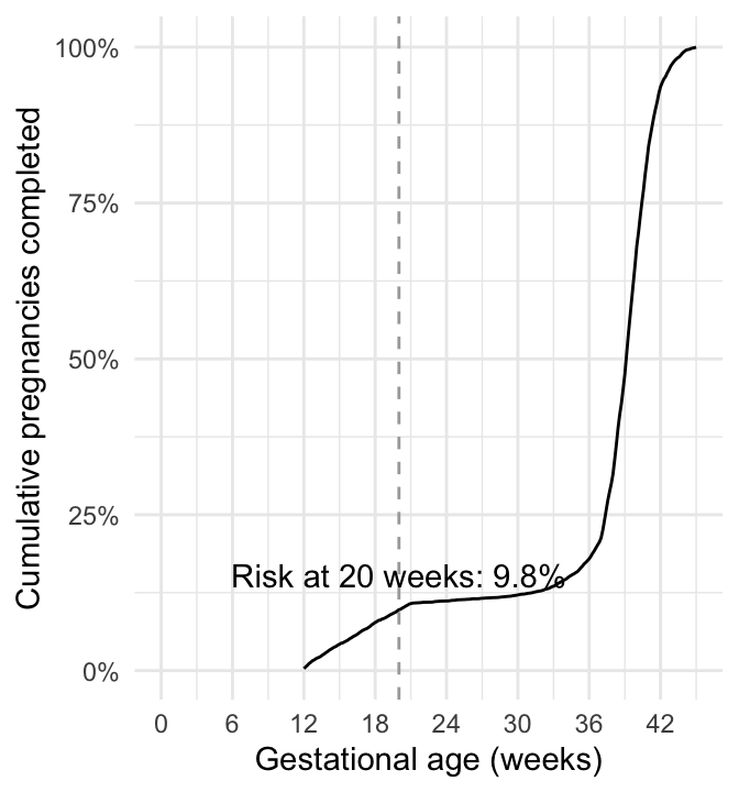
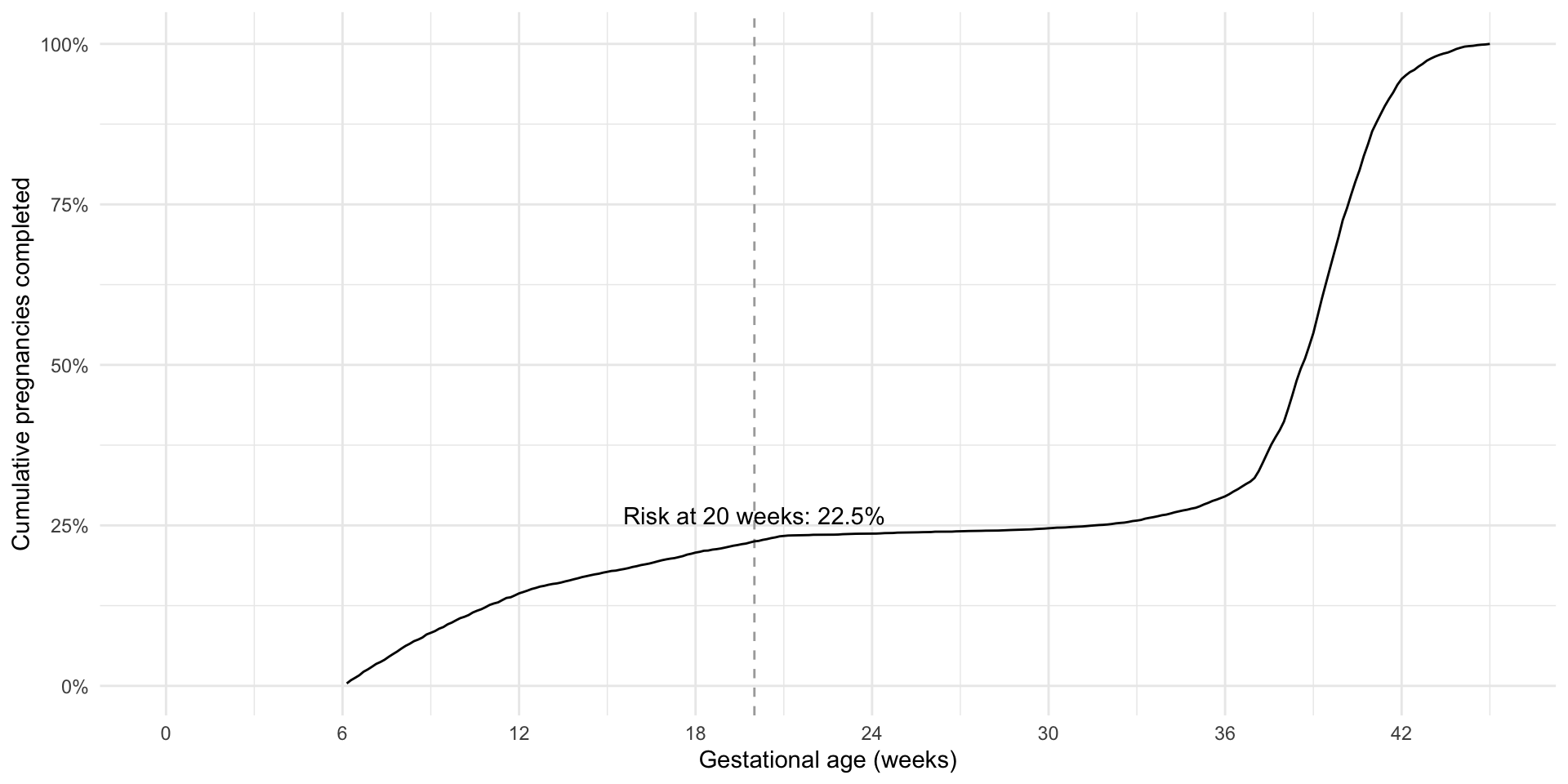
Obviously these are different! A lot of people have lost pregnancies between 6 and 12 weeks, so would not be included if enrollment started later.

summarise(dat_6wk, risk = mean(sab))

# A tibble: 1 × 1
   risk
  <dbl>
1 0.229

summarise(dat_12wk, risk = mean(sab))

# A tibble: 1 × 1
    risk
   <dbl>
1 0.0957

We can see this because the survival curves start at different times

Estimating survival curves in R

We can fit a Kaplan-Meier curve using the survfit() function from the survival package:

km_6wk <- survfit(Surv(gest_week, end_preg_event) ~ 1, data = dat_6wk)
km_12wk <- survfit(Surv(gest_week, end_preg_event) ~ 1, data = dat_12wk)

Unlike our generalized linear models, we don’t have a single variable on the left-hand side of the formula

• Instead, we use the Surv() function to specify the time-to-event outcome in the format Surv(time, event)
  • (This is why we had an end_preg_event variable that was 1 for everyone because we have complete follow-up)
  • The “1” on the right-hand side means we are not stratifying by any variables

Survival data in R

The data we are using looks like this:

dat_6wk |> 
    select(ID, gest_week, 
           end_preg_event, sab)

# A tibble: 9,604 × 4
      ID gest_week end_preg_event   sab
   <int>     <dbl>          <dbl> <dbl>
 1 46010     37.6               1     0
 2 76871     38.9               1     0
 3 67771     13.9               1     1
 4 33415     38.4               1     0
 5 32826     40.6               1     0
 6 64247     40.3               1     0
 7  3680      6.14              1     1
 8 29251     35                 1     0
 9 76826     41.9               1     0
10 82375     41.6               1     0
# ℹ 9,594 more rows

dat_12wk |> 
    select(ID, gest_week, 
           end_preg_event, sab)

# A tibble: 8,188 × 4
      ID gest_week end_preg_event   sab
   <int>     <dbl>          <dbl> <dbl>
 1 46010      37.6              1     0
 2 76871      38.9              1     0
 3 67771      13.9              1     1
 4 33415      38.4              1     0
 5 32826      40.6              1     0
 6 64247      40.3              1     0
 7 29251      35                1     0
 8 76826      41.9              1     0
 9 82375      41.6              1     0
10 30531      39.3              1     0
# ℹ 8,178 more rows

We plotted the survival curves (code in exercises)

What can we do about left truncation?

• In many settings, it won’t matter – we just need to be clear about what any absolute risk measures mean
• Pregnancy researchers are very familiar with the idea that pregnancy loss is much higher than we see in the data
• If we have a mix of enrollment times (with enrollment time random with respect to underlying risk of SAB), we can adjust for left-truncation using Surv(time_in, time_out, event) syntax:

km_mixed <- survfit(Surv(enroll, gest_week, end_preg_event) ~ 1, 
                    data = dat_mixed)

Interval survival data in R

km_mixed <- survfit(Surv(enroll, gest_week, end_preg_event) ~ 1, 
                    data = dat_mixed)

We are going to fit the model with this data:

# A tibble: 8,894 × 5
      ID enroll gest_week end_preg_event   sab
   <int>  <dbl>     <dbl>          <dbl> <dbl>
 1     1     12      40.6              1     0
 2     4      6      10.4              1     1
 3     5     12      41.7              1     0
 4    42      6      39.3              1     0
 5    52     12      39.6              1     0
 6    69      6      19.9              1     1
 7    80     12      39.1              1     0
 8    87     12      40                1     0
 9    91     12      39.6              1     0
10    97      6      39.1              1     0
# ℹ 8,884 more rows

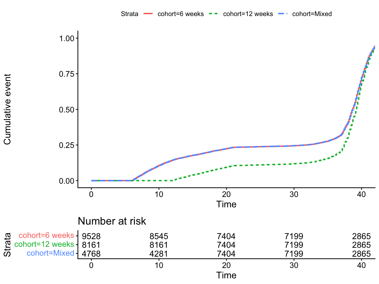
We get back our survival curves starting at the earliest enrollment time!

Compare risk tables

Differential left truncation

It will be a problem if enrollment time is related to the outcome (our absolute risk estimates will be biased) OR if enrollment time is related to the exposure, such that exposure groups have different enrollment patterns, and we don’t take this into account!

Bias due to differential left truncation: Howards, Hertz-Picciotto, and Poole (2007)

We’ll see how using target trial emulation can help us think through what questions make sense when we have left truncation

Exercises part 2

Chiu, Yu-Han, Mats J. Stensrud, Issa J. Dahabreh, Paolo Rinaudo, Michael P. Diamond, John Hsu, Sonia Hernández-Díaz, and Miguel A. Hernán. 2020. “The Effect of Prenatal Treatments on Offspring Events in the Presence of Competing Events: An Application to a Randomized Trial of Fertility Therapies.” Epidemiology 31 (5): 636. https://doi.org/10.1097/EDE.0000000000001222.

Gupta, Shalika, Laura B. Balzer, Moses R. Kamya, Diane V. Havlir, and Maya L. Petersen. 2024. “When Exposure Affects Subgroup Membership: Framing Relevant Causal Questions in Perinatal Epidemiology and Beyond.” arXiv. https://doi.org/10.48550/arXiv.2401.11368.

Howards, Penelope P., Irva Hertz-Picciotto, and Charles Poole. 2007. “Conditions for Bias from Differential Left Truncation.” American Journal of Epidemiology 165 (4): 444–52. https://doi.org/10.1093/aje/kwk027.

Rubin, Donald B. 2000. “Causal Inference Without Counterfactuals: Comment.” Journal of the American Statistical Association 95 (450): 435–38. https://doi.org/10.2307/2669382.

Stensrud, Mats J., Jessica G. Young, Vanessa Didelez, James M. Robins, and Miguel A. Hernán. 2020. “Separable Effects for Causal Inference in the Presence of Competing Events.” Journal of the American Statistical Association, June, 1–9. https://doi.org/10.1080/01621459.2020.1765783.

Young, Jessica G., Mats J. Stensrud, Eric J. Tchetgen Tchetgen, and Miguel A. Hernán. 2020. “A Causal Framework for Classical Statistical Estimands in Failure-Time Settings with Competing Events.” Statistics in Medicine 39 (8): 1199–1236. https://doi.org/10.1002/sim.8471.